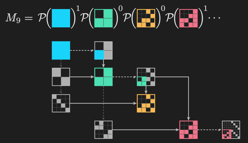
This post is going to start off describing what SZ Sequences are, and why I think the 4D shuffled-scrambled SZ Sequence should be the default sample sequence many people turn to when implementing something like a path-tracer. Then I’ll point to the open-source code that has them in Using SZ Sequences in Your Renderer.

After that, I suspect the rest of the post will only be interesting to maybe a dozen people. But it’s also where the real contribution is: the New Matrix Construction Algorithm section defines a procedure that’s much simpler and faster than Ahmed et al’s paper. And at the very end, in Hierarchical Faure-Niederreiter Sequences, I’ll expand the construction to other prime bases. The SZ Sequence is just the base-2 HFN Sequence.

Base-2 (0,2)-Sequences

A base-2 \((0,2)\)-sequence means for \(2^k\) points, they are stratified on every power-of-two 2D grid. For example, for the first 8 points, they are stratified on the 8x1 grid, the 2x4 grid, the 4x2 grid, and the 1x8 grid. This interactive diagram shows the stratification of a randomized base-2 \((0,2)\)-sequence.

This combination of stratification, but randomness within each grid cell, yields pretty much the lowest error you can get for a 2D progressive sample sequence for rendering.

So for two-dimensional sequences in a renderer, the state-of-the-art (and default choice for many renderers) are shuffled + scrambled base-2 \((0,2)\)-sequences. This is either called the (shuffled) PMJ02 sequence or Shuffled-Scrambled Sobol’ \((0,2)\)-sequence. Shuffling refers to a particular way of randomizing the order of the sample points (i.e. their indices), and scrambling refers to randomizing the positions of the points, without breaking their progressive stratification properties. Some more information about this is linked to from the Prerequisite Knowledge section.

As a side note, with shuffling and scrambling, PMJ02 and Sobol’ \((0,2)\) are actually identical: the probability density of getting any specific sequence is exactly the same. The two sequences are just different shuffles and scrambles of each other.

Higher Dimensionality

Given that \((0,2)\)-sequences are the best for 2D, what about if you want higher dimensions? When you’re writing a path-tracer, you need random numbers for each bounce, so your sampling really has 100s of dimensions. From what I know, production offline renderers typically use one of the two approaches:

1. Use the higher dimensional scrambled/stochastic Sobol’ sequence, up to a limited number of dimensions (4 or 5 is typical, I think).
2. “Shuffle” two scrambled/stochastic \((0,2)\)-sequences together to make a sequence with some weaker 4D stratification.

This gives 4D or 5D sequences, and then sequences “juxtaposed” with shuffling. Juxtaposing means that to make an 8D sequence, you simply combine two 4D sequences.

“Scrambling” is a technique to randomize the points within each grid cell, while “shuffling” is a technique to randomize the order of the points (the indices), and both can be done efficiently to preserve the stratification of the sequences. Shuffling is absolutely critical with juxtaposition, otherwise two 4D sequences will be highly correlated and may never converge, even for infinite samples.

The SZ Sequence

SZ Sequences, defined in SZ Sequences: Binary-Based (0, 2^q)-Sequences by Ahmed et al., are the best possible way to do Method #2.

Ahmed et al. talk about “SZ Sequences”, but in this post, I’m going to talk about “The Canonical SZ Sequence” or just “The SZ Sequence”, which I think is the simplest sequence to construct and the most obvious one to discover. And my belief is that all SZ Sequences can be obtained via Owen-shuffling and Owen-scrambling the canonical SZ Sequence.

So anyway, the SZ Sequence is actually an infinite-dimensional sequence, but for rendering you’ll most likely want to use only the first four dimensions. The properties are like this:

• Dimensions 0 and 1 form a base-2 \((0,2)\)-sequence.
• Dimensions 2 and 3 form a base-2 \((0,2)\)-sequence.
• Dimensions 0,1,2,3 form a base-4 \((0,4)\)-sequence.

Not only are the first and second pairs of dimensions the ideal stratification, but all 4 dimensions together also have the ideal stratification (which includes all lower dimensional projections). Not only that, but they have a high-dimensional stratification property where \(16^k\) points are always stratified on \(2^k \times 2^k \times 2^k \times 2^k\).

Consider the first 16 points, which have the following stratifications:

• First two dimensions: \([16 \times 1 \times 1 \times 1]\), \([8 \times 2 \times 1 \times 1]\), \([4 \times 4 \times 1 \times 1]\), \([2 \times 8 \times 1 \times 1]\), \([1 \times 16 \times 1 \times 1]\)
• Latter two dimensions: \([1 \times 1 \times 16 \times 1]\), \([1 \times 1 \times 8 \times 2]\), \([1 \times 1 \times 4 \times 4]\), \([1 \times 1 \times 2 \times 8]\), \([1 \times 1 \times 1 \times 16]\)
• Other 2D projections: \([4 \times 1 \times 4 \times 1]\), \([4 \times 1 \times 1 \times 4]\), \([1 \times 4 \times 4 \times 1]\), \([1 \times 4 \times 1 \times 4]\)
• High-dimensional: \([2 \times 2 \times 2 \times 2]\)

With higher point counts, the higher dimensional stratifications get filled out. For example at 64 points, all 3D projections have exactly one point in the 4x4x4 stratification. This is a bit harder to visualize, but maybe this helps.

It’s not really possible to do better than this in stratification - it’s much better than the 4D Sobol. And because it’s a base-2 sequence, the generation, scrambling, and shuffling can all be done with fast binary operations.

I mentioned that the SZ Sequence is infinite-dimensional. Well it actually has this expansive nesting property. The way it works is this. All even-odd pairs (disjoint groups of two) of dimensions are a base-2 \((0,2)\)-sequence, that is, any two dimensions \(2k, 2k+1\) for any integer \(k \geq 0\). All disjoint groups of 4, i.e. any \(4k, 4k+1, 4k+2, 4k+3\) are a base-4 \((0,4)\)-sequence. All disjoint groups of 16 are a base-16 \((0,16)\)-sequence. For example, the first 256 points are 2D stratified on the 16x16 grid for every pair of dimensions. Not just for the first 16 dimensions, but the 16 after that, and 16 after that, and so on. All disjoint groups of 256 dimensions are a base-256 \((0,256)\)-sequence. And so on, squaring the dimensionality each time, for an infinite number of dimensions.

The higher-dimensional forms of the SZ sequence probably wouldn’t be useful in a path-tracer. But they can still be very useful for offline purposes, such as precalculating some integrals. I suspect there may be other fields they are useful for (like in finance maybe, or physics).

The main contribution of this article over Ahmed et al.’s paper is presenting a significantly simpler and faster algorithm to construct the “generator matrices” for the SZ Sequences. This construction means you can pick any arbitrary dimension, say the \(2^{50}\)th dimension, and easily generate the points for that dimension - although that dimension would only be useful for 128-bit values (with 128x128 generator matrices).

Using SZ Sequences in Your Renderer

The reason that SZ Sequences are so phenomenal for a renderer is that we are often combining two inherently 2D sampling spaces anyway. For example, a 2D lens position and a 2D pixel position. Or a 2D light sample, and a 2D BRDF sample. So combining two optimal 2D sequences into an optimal 4D sequence is pretty awesome for rendering! In fact, I happened to see that OpenQMC - which is maintained primarily by Framestore - replaced the Sobol’ sequence with the SZ Sequence.

Now if you want to use randomized SZ Sequences in your renderer, there are fundamentally two approaches:

1. Use the Stochastic Generation technique to precalculate sample sequences. I’ve added SZ Sequences to the Stochastic Generation GitHub repo, so you can just use that!
2. Use Burley’s Hash-Based Scrambling + Shuffling. I’ve made a new SZ Sequences GitHub repo specifically for this purpose.

OpenQMC also takes the latter approach, and if you want to experiment with more sampling possibilities (and get some other benefits like screen-space blue-noise), then it’s a great way to go.

Prerequisite Knowledge

I’m not going to go over all the prerequisite knowledge here, but I would suggest reading the earlier sections of our paper “Stochastic Generation of (t,s) Sample Sequences”, at least up to Section 4.2. We made an effort to be formal but also to make it easy to understand the background information on how digital sequences are constructed. The important takeaway is that for a digital sample sequence, we need to construct a generator matrix for each dimension.

I also won’t cover how scrambling, shuffling, and stochastic generation work here. These are very important techniques to randomize these sequences for a renderer. If you want to learn more about them, check out the Stochastic Generation paper above, and I also strongly recommend “Practical Hash-based Owen Scrambling” because that is a more suitable implementation for a lot of renderers.

Backstory and AI Usage

Feel free to skip this section by the way. Nothing in it is referenced elsewhere.

Back when I was researching sampling in 2020 (prior to writing the Stochastic Generation paper, but shortly after figuring out an early form of the algorithm), I had the idea to search for generator matrices that could be useful for graphics. Most of these searches did not pan out, but I discovered what we now call SZ Sequences: two base-2 \((0,2)\)-sequences could be combined to form a base-4 \((0,4)\)-sequence. And four of these could be combined to form a base-16 \((0,16)\)-sequence, and so on. After publishing the Stochastic Generation paper, I was hoping to be able to find a direct construction of these matrices, but never did. It sat in the back of my mind as an open problem, but once I got my last job at Respawn, I didn’t really have enough time to dig further.

To my delight, Ahmed et al. published the SZ Sequences paper in 2025 on arXiv and later in ACM TOG (for SIGGRAPH Asia). They connected these sequences to the prime-power \((0,s)\) Niederreiter constructions from “Point Sets and Sequences with Small Discrepancy” (1987). I learned so much from their paper, I had no idea that prime-power finite fields could be represented as matrices of the base prime. But when I read their paper and thought about it more, I had a feeling that the construction was a bit more complex than it needed to be. It still required some searching (for an \(\alpha\) matrix), and also required sorting and rescrambling matrices. So I spent some time digging more, kind-of felt like there was a valid direction using polynomials and companion matrices to construct the alphabet, but I couldn’t get it.

Recently when Gemini 4 Argon came out, I thought I’d ask it to see if it could come up with a better construction. I told it the things I had already tried and the directions I was thinking… and it ran for about 10 minutes before it gave roughly the algorithm I’m describing in this article. It made some pretty amazing leaps and connected to some more obscure math theory (most of which I’m omitting here). After that I spent a lot of time understanding the exact algorithm, understanding the proof of why it works, and restructuring the algorithm to be easier to understand (and also slightly more efficient).

Like my other posts, the writing in this post is my own. I personally feel it’s important for me to understand (or think I understand) anything I put out there, and writing it myself is a way to enforce that. But like my last post, the diagrams are AI generated (with specific instructions from me), the written code is mostly AI, and I had it help with formatting and notation details of the math.

P.S. I actually have a bit of proof that I found the same sequences in 2020, this colab notebook, for which you can see the revision history from 2020. It was never meant to be read by anyone else, so it’s super messy, but it does show the search.

In any case, finding these sequences by brute-force was the easy part. I wouldn’t be surprised if Ahmed found them even earlier, and if others in the QMC community had found them before that. The work Ahmed et al. did to connect them to the Niederreiter construction and alpha matrices was the hardest part by far! Something that I probably never would’ve discovered on my own.

My main point in this Backstory section is to give a little insight into how these things develop over longer periods of time. Ahmed et al. in their paper wrote about the same thing (Section 2.5):

“We regard this as an excellent example of the community’s fast-paced learning cycles in analyzing and manipulating the inherently difficult-to-understand LD constructions. In this paper, we present an almost complete cycle from experimentation to the development of theoretical elements.”

I believe that sharing not just the end result but the research process is valuable to future researchers.

New Matrix Construction Algorithm

If you understand the digital method for generating QMC sequences, then you know that digital sequences are defined by their generator matrices for each dimension.

So now, I’ll present the new algorithm for generating the matrices for the SZ Sequence. Unlike the algorithm from the paper, this requires zero search, and no sorting or post-facto multiplication to restore the nesting. Also any arbitrary dimension’s matrix can be constructed very quickly, it’s not necessary to construct other dimensions (though it makes it a bit faster).

So we’ll look at how to construct a single matrix for an arbitrary dimension \(d\). Then we’ll look at generating all \(s\) dimensions at once, which is even more efficient since most of the work is shared across dimensions.

To construct the \(N \times N\) binary generator matrix \(M\) for dimension \(d\):

1. Initialize \(M = I_N\) (the \(N \times N\) identity matrix).
2. If \(d = 0\), return \(M\).
3. Let \(j = \lfloor \log_2(d) \rfloor\) be the index of the highest set bit of \(d\).
4. Generate the basis block matrices \(E_0, E_1, \dots, E_j\) (described below).
5. For \(i = 0 \dots j\):
   1. If bit \(i\) of \(d\) is set (i.e. (d >> i) & 1), multiply \(M\) on the right by the \(N \times N\) block-Pascal matrix \(\mathcal{P}(E_i)\): \(M \leftarrow M \cdot \mathcal{P}(E_i)\)
6. Return \(M\).

To generate the \(j + 1\) basis block matrices \(E_0, E_1, \dots, E_j\):

1. Initialize \(E_0 = \begin{bmatrix} 1 \end{bmatrix}\) and \(n = 1\).
2. While \(n \le j\):
   1. Set \(\beta = E_{n-1}\) (which is an \(n \times n\) matrix).
   2. For \(i = 0 \dots n - 1\) (while \(n + i \le j\)):
      1. Let \(E'_i\) be \(E_i\) repeated along the main diagonal to size \(n \times n\): \(E'_i = \begin{bmatrix} E_i & & 0 \\ & \ddots & \\ 0 & & E_i \end{bmatrix}_{n \times n}\)
      2. Construct the \(2n \times 2n\) basis matrix \(E_{n+i}\) as a \(2 \times 2\) block matrix with \(n \times\) blocks: \(E_{n+i} = \begin{bmatrix} 0_n & E'_i \\ \beta E'_i & E'_i \end{bmatrix}\)
   3. Set \(n \leftarrow 2n\).

And a block-Pascal matrix takes in an \(m \times m\) block matrix \(X\), and each \(m \times m\) block is defined as

Here is the Python implementation:

1
2
3
4
5
6
7
8
9
10
11
12
13
14
15
16
17
18
19
20
21
22
23
24
25
26
27
28
29
30
31
32
33
34
35
36
37
38
39
40
41
42
43
44
45
46
47
48
49
50
51
52
53
54
55
from math import comb
import numpy as np

def repeat_diagonal(block, n):
    m = len(block)
    k = n // m
    zero_m = np.zeros((m, m), dtype=int)
    return np.block([
        [block if i == j else zero_m for j in range(k)]
        for i in range(k)
    ])

def block_pascal(block, N):
    m = len(block)
    num_blocks = N // m
    powers = [np.identity(m, dtype=int)]
    for _ in range(num_blocks - 1):
        powers.append(np.matmul(powers[-1], block) % 2)

    P = np.zeros((N, N), dtype=int)
    for i in range(num_blocks):
        for j in range(i, num_blocks):
            if comb(j, i) % 2 == 1:
                P[i*m : (i+1)*m, j*m : (j+1)*m] = powers[j - i]
    return P

def generate_basis_matrices(num_matrices):
    basis_matrices = [np.array([[1]], dtype=int)]
    n = 1
    while n < num_matrices:
        beta = basis_matrices[n - 1]
        zero_n = np.zeros((n, n), dtype=int)
        for i in range(n):
            if n + i >= num_matrices:
                break
            E_enlarged = repeat_diagonal(basis_matrices[i], n)
            E_next = np.block([
                [zero_n,                         E_enlarged],
                [np.matmul(beta, E_enlarged) % 2, E_enlarged]
            ])
            basis_matrices.append(E_next)
        n *= 2
    return basis_matrices

def generate_sz_matrix(dim, N=32):
    M = np.identity(N, dtype=int)
    if dim == 0:
        return M

    num_basis = dim.bit_length()
    basis_matrices = generate_basis_matrices(num_basis)
    for i in range(num_basis):
        if (dim >> i) & 1:
            M = np.matmul(M, block_pascal(basis_matrices[i], N)) % 2
    return M

Now, there are a bunch of different ways to make this more efficient, I’ll mention two specifically:

1. For all practical purposes, what we really care about are the \(j+1\) Pascal matrices. These can be precalculated, like say the first 16 matrices, which makes it easy to generate any of the first \(2^{16}\) dimensions.
2. There is a mathematical property that \(\mathcal{P}(A)\mathcal{P}(B) = \mathcal{P}(A + B)\) if \(A\) and \(B\) commute (\(AB = BA\)). For any \(E_i\) matrices of the same size, within our finite field, they do commute. In this case, rather than multiply the Pascal matrices, you add the basis matrices before constructing the Pascal matrices. In a fast C++ implementation, this could work out to a single xor per column or row (if they were stored as an integer).

With the Pascal matrices precalculated, it is very fast to generate an arbitrary one of these matrices, beyond any dimension you’d want for any practical problem. One thing to note: for a dimension \(d \geq 2^{16}\), it only makes sense to have \(64 \times 64\) (or larger) generator matrices: for \(2^{16} \le d < 2^{32}\), the highest basis block \(E_j\) (with \(16 \le j \le 31\)) is \(32 \times 32\), so a \(32 \times 32\) block-Pascal matrix \(\mathcal{P}(E_j)\) consists of only a single \(I_{32}\) block on the diagonal (making it the identity matrix). You need at least \(N = 64\) so that \(\mathcal{P}(E_j)\) is at least a \(2 \times 2\) grid of \(32 \times 32\) blocks and actually includes \(E_j\) in the upper-right block.

Generating Multiple Matrices

This might be obvious, but if you want to generate a large group of these matrices, there’s a lot of work that’s repeated. As I mentioned you can precalculate the Pascal matrices, and on top of that, every time you double the array of generator matrices, you just need to multiply every previous generator matrix by the next Pascal matrix. Using the previous Python code, it just looks like this:

1
2
3
4
5
6
7
8
9
10
11
12
13
14
15
def generate_sz_matrices(num_dims, N=32):
    matrices = [np.identity(N, dtype=int)]
    if num_dims <= 1:
        return matrices[:num_dims]

    num_basis = (num_dims - 1).bit_length()
    basis_matrices = generate_basis_matrices(num_basis)
    pascal_matrices = [block_pascal(E_i, N) for E_i in basis_matrices]

    for P in pascal_matrices:
        matrices += [
            np.matmul(M, P) % 2
            for M in matrices[:num_dims - len(matrices)]
        ]
    return matrices

This takes only a single matrix multiplication to generate each new matrix, with log(dimensions) Pascal matrices calculated up front.

Why This Works (Informal Proof)

Definitions

Okay let’s start with a little semi-formal math notation. For an \(m \times m\) block matrix \(X\), let \(\mathcal{P}(X)\) be the \(N \times N\) upper-triangular block-Pascal matrix partitioned into \(m \times m\) blocks, with each block \(\mathcal{P}(X)_{i,j}\) (for \(0 \le i \le j\)) given by

where \(X^0 = I_m\), and \(\mathcal{P}(X)_{i,j} = 0_m\) for \(i > j\). This looks like:

For \(i > 0\), let \(k = \lfloor \log_2(i) \rfloor\) and \(n = 2^k\). Then \(E_i\) is a \(2n \times 2n\) basis matrix defined recursively from \(E_0 = \begin{bmatrix} 1 \end{bmatrix}\) as

where \(E'_{i-n}\) is \(E_{i-n}\) repeated along the main diagonal to size \(n \times n\).

Let \(b(i)\) be the binary decomposition of an integer \(i\) into bits \(c_0, c_1, \dots \in \{0, 1\}\) such that

Finally, the \(N \times N\) generator matrix \(M_d\) for dimension \(d\) with binary decomposition \(b(d) = (c_0, c_1, \dots)\) is simply

Note that each subsequent multiplication must be a right-multiplication.

4-Dimensional Case

So we’ll start by looking at the first 4 dimensions to get an intuition for why this works. The first four dimensions are specifically

Now let’s compare this to the classic Niederreiter construction for a base-4 \((0,4)\)-sequence:

where \(I_2 = \begin{bmatrix} 1 & 0 \\ 0 & 1 \end{bmatrix}\) and \(\alpha = \begin{bmatrix} 0 & 1 \\ 1 & 1 \end{bmatrix}\)

Now it turns out that \(E_1 = \alpha\), so \(M_0 = \widetilde{M}_0\) and \(M_2 = \widetilde{M}_2\) are already the same. I’m not going to fully work this out, but it’s possible to factor out our matrices in the following way:

where \(\mathcal{U}\) is the block-diagonal matrix that repeats \(U = \begin{bmatrix} 1 & 1 \\ 0 & 1 \end{bmatrix}\) along the main diagonal:

Now the important observation here is that this \(\mathcal{U}\) matrix will effectively scramble within a base-4 group of stratifications. This scrambling is a subset of Owen’s scrambling in base-4, and doesn’t break or change any \((t,s)\)-sequence properties in base-4, but it “fixes” the stratifications in base-2 to form the two base-2 \((0,2)\)-sequences. So our new construction is also a \((0,4)\)-sequence.

Now we also know that \(M_0 = I\) and \(M_1 = \mathcal{P}(E_0)\) form a base-2 \((0,2)\)-sequence, this is the classic Sobol’ and Faure construction. \(M_2 = M_0\mathcal{P}(E_1)\) and \(M_3 = M_1\mathcal{P}(E_1)\), and \(\mathcal{P}(E_1)\) is a non-singular upper-triangular (NUT) matrix. Faure and Tezuka showed in “Another random scrambling of digital (t,s)-sequences” (2002) that taking a \((t,s)\)-sequence and right-multiplying every matrix by a NUT matrix preserves the \((t,s)\) property, it’s really just a base-2 reshuffling of the indices. So \(M_2\) and \(M_3\) also form a base-2 \((0,2)\)-sequence.

16-Dimensional Case

Now to extend to 16 dimensions, the argument is similar. The \(M\) SZ Sequence matrices can be factored out to be left-scrambles of the \(\widetilde{M}\) matrices of Niederreiter’s construction:

where the \(\mathcal{U}_0\) and \(\mathcal{U}_1\) matrices are still block-diagonal matrices, where the blocks are \(4 \times 4\) NUT matrices. This is a valid base-16 scrambling that does not affect the \((0,16)\)-sequence properties of the sequence.

Minor notation detail: the first four \(\widetilde{M}_i\) matrices in this 16-dimensional case are not the same as the ones in the 4-dimensional case. I’m just using this as a shorthand to mean the Niederreiter matrices.

Generalization

Generally speaking, every matrix of this SZ Sequence is a similar block-diagonal left-scrambling of the matrices from the Faure-Niederreiter constructions. I’m not going to formally prove this in this blog post, but that’s the intuition for why this works.

Hierarchical Faure-Niederreiter Sequences

It turns out that this “hierarchical” construction is not limited to binary matrices, we can extend it to other prime bases. This is likely not very useful for computer graphics, but might be more interesting to QMC folks. I’ll refer to these as Hierarchical Faure-Niederreiter Sequences or HFN sequences, where SZ are the base-2 HFN sequences.

Specifically a Hierarchical Faure-Niederreiter Sequence in prime base \(p\) is an infinite-dimensional sequence such that for any integers \(k \geq 0\), \(q \geq 0\), we have a base \(b = p^{p^q}\), so that the coordinates for dimensions \(kb, \dots, (k+1)b-1\) form a base-\(b\) \((0,b)\)-sequence. Sometimes these are called “aligned dimensions” or “disjoint groups” of dimensions.

The generalized construction goes like this, for dimension \(d\), with a prime base \(p\):

1. Initialize \(M = I_N\) (the \(N \times N\) identity matrix).
2. If \(d = 0\), return \(M\).
3. Calculate the base-\(p\) representation of \(d\), i.e. the digits \(c_0, c_1, \dots, c_j \in \{0, 1, \dots, p - 1\}\) such that \(d = \sum_{i=0}^{j} c_i p^i\), where \(j = \lfloor \log_p(d) \rfloor\) is the index of the highest non-zero digit.
4. Generate the basis block matrices \(E_0, E_1, \dots, E_j\) (described below).
5. For \(i = 0 \dots j\): \(M \leftarrow M \cdot \mathcal{P}(E_i)^{c_i} \pmod p\)
6. Return \(M\).

To generate the \(j + 1\) basis block matrices \(E_0, E_1, \dots, E_j\):

1. Initialize \(E_0 = \begin{bmatrix} 1 \end{bmatrix}\) and \(n = 1\).
2. While \(n \le j\):
   1. Set \(\beta = E_{n-1}\) (which is an \(n \times n\) matrix).
   2. Let \(\alpha\) be a \(pn \times pn\) matrix (a \(p \times p\) grid of \(n \times n\) blocks), with \(\beta\) in the bottom-left, \(I_n\) just to the right of \(\beta\), and the upper-right portion of the matrix is the identity matrix (I think this is called the super-diagonal): \(\alpha = \begin{bmatrix} 0_n & I_n & 0_n & \cdots & 0_n \\ 0_n & 0_n & I_n & \cdots & 0_n \\ \vdots & \vdots & \vdots & \ddots & \vdots \\ 0_n & 0_n & 0_n & \cdots & I_n \\ \beta & I_n & 0_n & \cdots & 0_n \end{bmatrix}_{pn \times pn}\)
   3. For \(m = 1 \dots p - 1\):
      1. For \(i = 0 \dots n - 1\) (while \(mn + i \le j\)):
         1. Let \(E'_i\) be \(E_i\) repeated along the main diagonal to size \(pn \times pn\): \(E'_i = \begin{bmatrix} E_i & & 0 \\ & \ddots & \\ 0 & & E_i \end{bmatrix}_{pn \times pn}\)
         2. Construct the \(pn \times pn\) basis matrix \(E_{mn+i}\) as: \(E_{mn+i} = \alpha^m E'_i \pmod p\)
   4. Set \(n \leftarrow pn\).

And again, the block-Pascal matrix \(\mathcal{P}(X)\) for prime base \(p\) is defined with each block as:

In this generalized construction, you might notice that \(\alpha\) is a companion matrix for a monic polynomial, specifically \(x^p - x - \beta = 0\) over the previous (nested) field. I haven’t gotten into it in this post, but that’s the secret of how this construction was derived.

Anyway here is the full Python code for HFN sequences, both for individual matrices of an arbitrary dimension, and for the first num_dims matrices.

1
2
3
4
5
6
7
8
9
10
11
12
13
14
15
16
17
18
19
20
21
22
23
24
25
26
27
28
29
30
31
32
33
34
35
36
37
38
39
40
41
42
43
44
45
46
47
48
49
50
51
52
53
54
55
56
57
58
59
60
61
62
63
64
65
66
67
68
69
70
71
72
73
74
75
76
77
78
79
80
81
82
83
84
85
86
87
88
89
90
91
92
93
94
95
96
97
98
99
100
101
102
103
from math import comb
import numpy as np

def repeat_diagonal(block, n):
    m = len(block)
    k = n // m
    zero_m = np.zeros((m, m), dtype=int)
    return np.block([
        [block if i == j else zero_m for j in range(k)]
        for i in range(k)
    ])

def matrix_power_mod(matrix, exp, p):
    result = np.identity(len(matrix), dtype=int)
    for _ in range(exp):
        result = np.matmul(result, matrix) % p
    return result

def block_pascal(block, N, p):
    m = len(block)
    num_blocks = N // m
    powers = [np.identity(m, dtype=int)]
    for _ in range(num_blocks - 1):
        powers.append(np.matmul(powers[-1], block) % p)

    P = np.zeros((N, N), dtype=int)
    for i in range(num_blocks):
        for j in range(i, num_blocks):
            coeff = comb(j, i) % p
            if coeff != 0:
                P[i*m : (i+1)*m, j*m : (j+1)*m] = (coeff * powers[j - i]) % p
    return P

def make_alpha_matrix(beta, p):
    n = len(beta)
    zero_n = np.zeros((n, n), dtype=int)
    ident_n = np.identity(n, dtype=int)
    blocks = [[zero_n for _ in range(p)] for _ in range(p)]
    for r in range(p - 1):
        blocks[r][r + 1] = ident_n
    blocks[p - 1][0] = beta
    blocks[p - 1][1] = ident_n
    return np.block(blocks)

def generate_basis_matrices(num_matrices, p):
    basis_matrices = [np.array([[1]], dtype=int)]
    n = 1
    while n < num_matrices:
        beta = basis_matrices[n - 1]
        alpha = make_alpha_matrix(beta, p)
        for m in range(1, p):
            alpha_m = matrix_power_mod(alpha, m, p)
            for i in range(n):
                if m * n + i >= num_matrices:
                    break
                E_enlarged = repeat_diagonal(basis_matrices[i], p * n)
                E_next = np.matmul(alpha_m, E_enlarged) % p
                basis_matrices.append(E_next)
        n *= p
    return basis_matrices

def generate_hfn_matrix(dim, p=2, N=32):
    M = np.identity(N, dtype=int)
    if dim == 0:
        return M

    digits = []
    temp = dim
    while temp > 0:
        digits.append(temp % p)
        temp //= p

    num_basis = len(digits)
    basis_matrices = generate_basis_matrices(num_basis, p)
    for i, c_i in enumerate(digits):
        if c_i != 0:
            P_i = block_pascal(basis_matrices[i], N, p)
            M = np.matmul(M, matrix_power_mod(P_i, c_i, p)) % p
    return M

def generate_hfn_matrices(num_dims, p=2, N=32):
    matrices = [np.identity(N, dtype=int)]
    if num_dims <= 1:
        return matrices[:num_dims]

    num_basis = 0
    temp = num_dims - 1
    while temp > 0:
        num_basis += 1
        temp //= p

    basis_matrices = generate_basis_matrices(num_basis, p)
    pascal_matrices = [block_pascal(E_i, N, p) for E_i in basis_matrices]

    for P in pascal_matrices:
        prev_matrices = list(matrices)
        for c_i in range(1, p):
            P_pow = matrix_power_mod(P, c_i, p)
            matrices += [
                np.matmul(M, P_pow) % p
                for M in prev_matrices[:num_dims - len(matrices)]
            ]
    return matrices