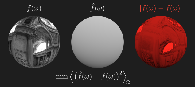
Ever since I first heard of spherical harmonics as an approximation in computer graphics, I have felt that the way they are explained is too complicated. Sometimes the explanations assume a bunch of math knowledge that isn’t really necessary, and they tend to be very abstract. Other times they show something complex and through a lot of effort end up simplifying them to something usable. In addition to making it harder to learn, I think those approaches to SH can lead to misapplication. SH introductions often have discussion about certain SH artifacts (ringing and negative values), but ignore another class of common issues.

In this post, what we’re going to do is start with a common problem in graphics, solve it as simply as we can using tools that I think many programmers are familiar with, and end up getting something that is equivalent to SH approximations. The aim of this post is to teach SH for graphics in a more intuitive way, but even if you already know how to use SH in graphics, I hope that this approach will give a new perspective.

AI Disclaimer

All of the prose writing in this article is my own, not AI. I did the derivations by hand but then asked AI to convert to proper KaTeX formatting and fix inconsistent notation, and the AI filled out a few other things (like the Orthogonal Form rules). However all of the diagrams were implemented by AI (with multiple iterations), and I also incorporated feedback and error-corrections from AI.

A Spherical Function

So let’s start with the engineering problem. We have a whole bunch of values that are oriented in different directions. In graphics, a common example of this is the incoming light (radiance) at a particular point in space, which has a different value in different directions. For this one specific point in space, we can call these values a function \(f(\omega)\), where omega \(\omega\) is a direction, with components \(\langle \omega_x, \omega_y, \omega_z \rangle\) and \(\omega_x^2 + \omega_y^2 + \omega_z^2 = 1\). In other words, it’s a unit vector.

This visualization is a simple example of what this function might look like. You can see the spherical directions from the surface normal, or view the incoming light via a reflection (bounced rays) in a chrome ball.

For a given direction \(\omega\), calculating the value \(f(\omega)\) is expensive. It could mean ray-tracing, path-tracing, or rasterizing a pixel. In real-time rendering for a game, you typically don’t want to fully calculate a reflection value for every point that you want to shade. Alternatively, you can pre-render a high resolution version of the spherical function, possibly storing in a cubemap or an octahedral map. But this requires a lot of memory for many points in space.

If we don’t need very high resolution, instead we may want to store a fast very low resolution approximation, we’ll call \(\hat{f}\). Note that \(\hat{f}\) is called “F hat” and the hat is common notation for approximations in statistics.

A 6-pixel (one for each face) cubemap or 8-value octahedral map works in many cases, but there are downsides which I won’t go into here.

A Linear Approximation

So instead, let’s come up with a mathematical approximation \(\hat{f}(\omega)\) for our function \(f(\omega)\). A linear model like this is just about the simplest reasonable approximation that I can think of (aside from a flat constant):

Where we will precalculate and store our four coefficients: \(c_0, c_x, c_y, c_z\).

It might be obvious that you can think of the \(c_0\) term as an overall intensity, and the \(c_x, c_y, c_z\) as a directional intensity, for a particular direction. And if the length of the \(\langle c_x, c_y, c_z \rangle\) vector is larger than \(c_0\), you can get negative values (which will render in red below).

So how do we get these four coefficients? A quick idea might be to find the coefficients \(c_0, c_x, c_y, c_z\). that minimize the (sum/average/integrated) square error \((\hat{f}(\omega) - f(\omega))^2\) against the original function or a high-resolution version. In other words, a good old fashioned linear regression. In this Python code we’ll sample some random directions and regress on those.

1
2
3
4
5
6
7
8
9
10
11
12
13
def encode_linear_coefficients(spherical_fn, num_dirs=8192, seed=None):
    dirs = generate_uniform_sphere_dirs(num_dirs, seed=seed)
    spherical_values = [spherical_fn(dir) for dir in dirs]

    # Calculate four linear coefficients for model with a constant
    # Construct the design matrix A: [1, x, y, z]
    A = np.hstack((np.ones((num_dirs, 1)), dirs))
    y = np.array(spherical_values)

    # Solve for least squares: A * c = y
    coefficients, _, _, _ = np.linalg.lstsq(A, y, rcond=None)

    return coefficients

These coefficients give us our fast, low-memory spherical approximation.

Well, we pretty much just reinvented spherical harmonic approximations! This is most likely something countless people have done without even realizing that what they did was equivalent to using SH.

Maybe it would be more accurate to say that this is a valid, though inefficient, implementation of a specific SH approximation. We would call this an \(l = 1\), or L1, spherical harmonics approximation, where “\(l\)” is the degree of the polynomial. You can also have an \(l = 0\) SH approximation, with a single constant like \(\hat{f}(\omega) = c_0\).

Higher \(l\) values will store coefficients for higher degrees of polynomials, for example \(l = 2\) includes coefficients for \(x^2\), \(xy\), \(xz\), \(y^2\), etc. Higher degree polynomials have a bit of extra complexity we’ll talk about later, but it’s still just a basic linear model, with a least squares fit!

Spherical harmonic approximations are actually nearly the blandest approximation model you could think of to represent a spherical function. If this is the first time you’re learning about SH, you might be thinking… why do we even use a special name for a basic linear model?

You may notice that I’ve been saying SH approximations rather than just SH. A big part of why we have a special name is the difference between the mathematical construct (spherical harmonics) and the application of them (SH approximations). Also part of the answer is due to the history of the application of SH to graphics, and due to the relationships with other things in math.

But there are two interesting properties of SH approximations that make them special compared to other linear models:

1. Very fast and simple calculation of the coefficients (encoding)
2. Very fast convolutions of the spherical harmonic approximation

In graphics, performance is really important, so being able to do these things fast is a big part of why SH approximations are used at all.

As I’ll show shortly, the first property is because we are optimizing least squares over the uniformly weighted unit sphere, rather than any arbitrary distribution of x,y,z values.

Fast Calculation of the (L1) Linear Model Coefficients

The calculation of the coefficients is often called “encoding”. In a machine learning context this would often be called regression or fitting or learning or maybe compressing or mayyybe training.

When it comes to spherical harmonics, the fast method of encoding is specifically called projection.

Then evaluating the approximation function \(\hat{f}\) I’ll usually call reconstruction, but it could also be called decoding. In an ML context it might be called inference or estimation (or prediction, but that’s not really appropriate here, since we’re approximating something that’s known, rather than predicting something unknown).

We’re going to derive the fast encoding from scratch, for both the \(c_0\) term and the \(c_x\) term. The \(c_y\) and \(c_z\) terms are basically the same as \(c_x\). The derivation involves a small amount of calculus, but if you want, you can skip the L1 Encoding Derivation section, and go to L1 Encoding Rules (Projection).

L1 Encoding Derivation

Typically to minimize a function with multiple parameters, you’d need to jointly minimize every parameter. But let’s see what happens if we start by optimizing just \(c_0\) on its own.

We want to find the \(c_0\) that minimizes least squares errors. This is written as:

In this case, the integral over big-omega \(\Omega\) means we’re integrating over the sphere, and the little omega \(\omega\) represents a direction.

But rather than using spherical integrals, we’re going to switch to spherical averages (means), because minimizing the integral of squared error is the same as minimizing the average squared error. The notation I will use for a spherical average uses the angle brackets \(\langle \, \rangle_\Omega\). The more standard notation drops the \(\Omega\) subscript, but I think it’s clearer to keep it, especially to distinguish between vectors which also use the angle brackets.

Formally, the average is the same as the integral divided by the surface area of the sphere:

Doing this means that we can ignore the surface area of the sphere, which makes the math and programming easier.

I am not the first person to use spherical averages to simplify SH, and I think Graham Hazel did the best job fleshing this out, but I’ll link to that article in the Bridging the Gap section. Anyway, so we are trying to solve:

To find a minimum, we need to find the value of \(c_0\) such that the first derivative of this is zero.

Typically to minimize you’d also worry about local minima or finding maxima, but as we’ll see, there is only one solution here - the function is convex.

The derivative of an average is the average of the derivative:

Typical power and chain rule:

Now let’s focus on \(\frac{\partial(\hat{f}(\omega) - f(\omega))}{\partial c_0}\).

\(\frac{\partial f(\omega)}{\partial c_0}\) is zero, because \(c_0\) is unrelated to the original function.

Expanding \(\hat{f}(\omega)\), we have \(\frac{\partial(c_0 + c_x \omega_x + c_y \omega_y + c_z \omega_z)}{\partial c_0}\), which is simply \(1\).

Plug this back a few lines up:

Divide by 2, plug in the definition of \(\hat{f}(\omega)\) again, and separate all the average terms, and we have this:

Now the average \(\langle c_0 \rangle_\Omega\) is of course \(c_0\), it’s a constant. \(\langle c_x \omega_x \rangle_\Omega\) is 0, because it’s symmetrically distributed over a sphere (for every \(\omega_x\) value, there is also a \(-\omega_x\) value), and same for the other two terms. So we get this wonderfully intuitive and easy to calculate value.

The constant is just the average value of our function over the whole sphere!

Not only that, as we alluded to earlier, the optimal \(c_0\) value is not dependent on any of the other coefficients - they can be optimized independently.

Now let’s do the same for \(c_x\)…

Like the previous derivation, we would first take the derivative and set it to zero. And then starting with the chain rule and power rule and move the average outside the derivative:

Focusing on the inner derivative term, again we separate the terms, such that

\(\frac{\partial f(\omega)}{\partial c_x}\) is still zero, because \(c_x\) is unrelated to the original function.

\(\frac{\partial\hat{f}(\omega)}{\partial c_x} = \frac{\partial(c_0 + c_x \omega_x + c_y \omega_y + c_z \omega_z)}{\partial c_x}\) and that is simply \(\omega_x\), because it’s the only term with \(c_x\).

So now we have:

or

Expanding \(\hat{f}(\omega)\) and separating the average terms:

Because of spherical symmetry, every average term is zero except the \(\omega_x^2\) one, because \(\omega_x^2\) is non-negative everywhere, which simplifies to:

Because \(\omega\) is a unit vector, we know that the length and length squared are one:

So we can also say that the average squared values add up to 1:

Since a sphere is symmetrical for all the three axes, the averages are all the same: \(\langle \omega_x^2 \rangle_\Omega = \langle \omega_y^2 \rangle_\Omega = \langle \omega_z^2 \rangle_\Omega\), and we can substitute that in, so \(3 \langle \omega_x^2 \rangle_\Omega = 1\). That gives us:

Now you start to get a sense for why this is called “projection”. It looks like projecting the function onto the \(\omega_x\) value, with a scale.

L1 Encoding Rules (Projection)

Now we have our super fast and easy encoding of coefficients for our linear model - projection.

And a little Python code can be written to estimate this numerically, like:

1
2
3
4
5
6
7
8
9
10
11
def encode_linear_coefficients_fast(spherical_fn, num_dirs=8192, seed=None):
    dirs = generate_uniform_sphere_dirs(num_dirs, seed=seed)

    mean = np.array([0.0, 0.0, 0.0, 0.0])
    for i, dir in enumerate(dirs, 1):
        value = spherical_fn(dir)
        sample = np.array([1.0, 3.0*dir[0], 3.0*dir[1], 3.0*dir[2]]) * value
        # Welford's method for computing the mean
        mean += (sample - mean) / i

    return mean

For a long time I found spherical harmonics a bit scary. Personally, derived this way, I find it hard to imagine a simpler spherical approximation to understand and implement! It’s a single line of code to evaluate \(\hat{f}(\omega)\), and only a few lines of code to encode the coefficients. And on top of that, it’s doing something that many engineers are already familiar with, just a simple linear model with least squares, plus a trick to encode the coefficients in a faster way.

Questioning Our Assumptions

Now that we’ve derived the fast encoding, let’s reconsider some important assumptions we made for this fast encoding to be the least-squares solution.

1. Our reconstruction function is \(\hat{f}(\omega) = c_0 + c_x \omega_x + c_y \omega_y + c_z \omega_z\)
2. We want to minimize least squares error, not some other error.
3. Our function or optimization domain is uniformly distributed around the unit sphere, in all directions.

Typical applications of spherical harmonics in graphics violate at least one of these assumptions, sometimes two, often all three. Even when the assumptions are violated, spherical harmonics are still usually pretty good in practice, but sometimes the issues can be significant.

Assumption 1 Violations

The first assumption might seem comically obvious - of course the encoding only works for the reconstruction function that it was derived with! But virtually all SH implementations in graphics violate it. For one thing, there are improvements to spherical harmonics that use different forms of reconstruction, i.e. completely different models, like the Geomerics reconstruction (this also includes a convolution).

But even the most vanilla implementations of SH almost always add a clamp to the reconstruction fuction / approximation model to prevent negative lighting values:

The L1 Encoding Rules (projection) are a naive linear fit that does not take the clamp into account, and so those coefficients are not actually the optimal solution for the clamped model. This is not necessarily a big problem, and I’ve even seen attempts to address it introduce worse problems. But it is possible to do better in specific cases by minimizing error for the clamped function.

A specific graphics example might be when SH approximations are used to represent reflected/outgoing radiance from a Lambertian/diffuse BRDF. In this case, the direction \(\omega\) used is a surface normal (because for a given normal, light is equally reflected in all visible directions with this BRDF). If our lighting is a simple directional light, we can perfectly represent the Lambertian reflected light using the clamped function, with zero error. But naive SH projection is overly soft, because it’s minimizing error for the wrong reconstruction function.

Assumption 2 Violations

I won’t go into too much detail here, but least squares error is rarely ideal for graphics applications. The eye is much more sensitive to small changes in light in a dark room than in bright sunlight. So a relative (pseudo-logarithmic) error is usually better, and there are even better perceptual error metrics depending on what you know about your scene. This might be something I tackle in a future blog post, but for better error functions you might need to use gradient descent or other techniques to get the optimal solutions.

Assumption 3 Violations

Finally, IMO the most important mistake is using SH projection (the fast encoding rules) when your function domain is not a sphere. A very common domain is a hemisphere, for example when generating directional lightmaps. This can actually lead to meaningful bias, ending up too bright even for a completely flat surface where we should be matching non-directional lightmaps.

In addition to hemispherical domains, sometimes you might want to do things like optimize lighting for the points on the surface of a model. A good fallback here is to use standard linear regression like in the very first Python example.

In practice, these assumption violations may or may not be important problems in your application, but I have seen significant improvements to visual quality by addressing them.

Convolution

Let’s say we have an L1 spherical harmonic approximation, encoded with our 4 coefficients \(c_0, c_x, c_y, c_z\). Then we have a symmetric spherical convolution \(g(f)\), which could do something like “blur” or “sharpen” the approximation.

I’ll spoil the surprise before doing the derivation this time. It turns out that for a given convolution \(g(f)\), we can simply precompute 2 coefficient factors, one for \(c_0\) and another that multiplies \(c_x, c_y, c_z\). For example, let’s say we have a Lambertian (diffuse) BRDF. For a given surface normal \(n\), to “convolve” from incoming radiance for every direction to the reflected radiance (which is uniform across all reflection directions), you just multiply the \(c_x, c_y, c_z\) components by \(2/3\)! This is taking into account the typical \(\frac{1}{\pi}\) BRDF constant.

Now we’ll derive this rule for convolutions, for \(c_0\) at least. Let’s say that a convolution takes in a spherical function or data, a direction, and outputs a value that is a weighted integral of the original spherical function.

Note that this convolution kernel \(h\) doesn’t depend on two arbitrary directions, only the dot product (i.e. angle) between them. This means the convolution is symmetric around the direction \(n\), and the same everywhere around the sphere.

Now we can also express our \(c_0\) encoding rule as an integral, for example

We want to get the encoding of our convolution:

We can flip the nesting order of the integrals (think of them just like sums):

And pull \(f(\omega)\) out of the inner integral because it’s unrelated to \(\mathrm{d}n\)

Now \(\int_\Omega h(n \cdot \omega) \, \mathrm{d}n\) is a constant value, we’ll call it \(k_0\), so we have

Pull the \(k_0\) out of the integral, it’s a constant:

Which is simply

This might seem a bit mathy, but I think in plain English it’s intuitive. \(c_0\) is just the average intensity of our function over a sphere. A convolution multiplies the average intensity up or down, but that’s all it can do, and the multiplication amount is constant (it’s the integral of the weight of the convolution kernel over the sphere).

We can do basically the same rearrangements for the other coefficients, and in the end, we get very simple scale factors.

In other words, given any rotationally symmetric convolution \(g(f)\), we can precalculate two \(k\) values, let’s say \(k_0, k_{xyz}\). Then the convolved approximation \(g(\hat{f})(\omega)\) and the approximation of the convolution \(\widehat{g(f)}(\omega)\) are both just \(c_0 k_0 + c_x k_{xyz} \omega_x + c_y k_{xyz} \omega_y + c_z k_{xyz} \omega_z\).

Again, all of this is under the assumption that our integrals are uniformly oriented around a sphere. But if we’re working on, say, hemispheres or arbitrary surfaces, things can get more complicated.

I’ll add one other neat detail, which is that any linear transformation on a sphere (this could also include rotations, anisotropic convolutions, squishing, etc.) can be baked into an \(n \times n\) matrix for \(n\) spherical harmonic coefficients, and transforming an encoding is just a matrix multiplication. But a rotationally symmetric convolution is a special case where it’s a diagonal matrix.

Higher Degree Polynomials

Now let’s say we want to use second-degree polynomials (L2). We can add terms to our linear model to get this reconstruction function, which I’ll call “Fast Reconstruction Form” or FRF:

You might notice that \(c_{z^2} \omega_z^2\) is missing. This is because we know that this is a unit vector, so \(\omega_x^2 + \omega_y^2 + \omega_z^2 = 1\), and so \(\omega_z^2 = 1 - \omega_x^2 - \omega_y^2\), and those aspects are redundant with the coefficients \(c_0\), \(c_{x^2}\), and \(c_{y^2}\).

But if we want to find the encoding rules like we did for the L1 model, things get a little more complicated. We have two options for how to approach things:

Option 1: Keep reconstruction as cheap as possible, use the simple linear model given above (Fast Reconstruction Form). Option 2: Keep encoding simpler at a slight expense to reconstruction, and keep the coefficients independent (Orthogonal Form, which I’ll give below).

Let’s start with Option 1 because it’s more informative as to why it’s problematic. In practice I would typically use Option 2 in real-time graphics. But Option 1 I’d use in any situation where we’re actually doing gradient descent anyway (say, as part of some other ML model).

Fast Reconstruction Form (FRF) Issues

To understand why the encoding gets more complicated, we’ll do some math using a simpler model of only one axis:

We’ll now rederive the encoding rules for all three coefficients. Even though it’s only one axis, this is a little bit denser than the L1 derivation and I’m going to skip more within it, so feel free to jump ahead to the L2 Encoding Rules.

Again we start with taking the partial derivative and setting it equal to zero.

I’ll skip a few of the simple steps from before, application of the chain and power rules, dividing by two, and that \(\frac{\partial (\hat{f}(\omega) - f(\omega))}{\partial c_0}\) simplifies to \(1\), and we get

Moving terms around, and taking advantage of the knowledge that \(\langle \omega_x \rangle_\Omega = 0\), we get

As we can see, \(c_0\) is no longer a simple average of the function. It’s related to the value of \(c_{x^2}\). We’ll need to solve for this.

Next up is \(c_x\). I’m going to mostly skip this, because it ends up the same as in the L1 Encoding Derivation, due to the fact that every odd power of \(\omega_x\) has an average value of zero over the sphere, giving us:

Finally we have \(c_{x^2}\).

The first few steps work out again like this:

Before we showed that \(\langle \omega_x^2 \rangle_\Omega = \frac{1}{3}\). And we know that \(\langle \omega_x^3 \rangle_\Omega = 0\). I won’t derive this here, but \(\langle \omega_x^4 \rangle_\Omega = \frac{1}{5}\).

So this gives us

Now we have a linear system (two variables \(c_0\) and \(c_{x^2}\), two equations). Most general way to solve this is to reformulate it with a matrix form:

And this can be solved with Gaussian elimination, or inverting the matrix and multiplying on the left for both sides of the equation.

Finally for our one-axis model, we get this:

This doesn’t really help us with the multi-axis derivation directly, but it shows why this gets a bit more complicated. The different coefficients and “projections” now have interdependencies.

L2 (FRF) Encoding Rules

The encoding rules for the multi-axis FRF model require a longer derivation, but it’s more of the same, so I’ll just give the rules themselves:

Orthogonal Form

The Fast Reconstruction Form above means the encoding rules get a little bit uglier. You can also argue that the coefficients are less interpretable - before with L1 it was nice that \(c_0\) was a simple average over the unit sphere. This could mean, for example, that if you were developing a game with options for high-quality and very low-quality global illumination using spherical harmonics, you could just use \(c_0\) for the very low-quality version. But that’s no longer true.

To address these problems, we can change our reconstruction function to keep all the terms orthogonal, which practically means they won’t affect each other in encoding or convolution. This is mathematically the same model (it will give the same approximation), but the changed “features” or “columns” (as we’d call them in ML or stats) have been changed in a way that the minimum coefficients will have terms that cancel out.

Note that the coefficients have different subscripts now and the terms have been rearranged a bit, this is to be more consistent with typical spherical harmonic definitions. This is a bit hand-wavey - it might be nice to derive these specific forms rather than presenting them immediately - but I wasn’t sure if it would add much value to this post.

The important thing is that we get simpler and more consistent encoding rules:

Now we can see that there is a comforting similarity between the encoding and reconstruction, where we are still just “projecting” the original function onto each term of the reconstruction approximation, and multiplying by a constant.

Bridging the Gap

We’ve pretty much derived SH approximations from scratch now, so I want to end by highlighting how this approach differs from the typical one, and start to introduce the real mathematical definitions.

To recap here’s our L1 reconstruction equation:

And here’s our L1 encoding rules:

By contrast, a typical implementation of SH does this reconstruction:

With encoding as

If you plug the encoding values into the reconstruction, remembering that \(\int_\Omega f(\omega) \mathrm{d}\omega = 4 \pi \langle f(\omega) \rangle_\Omega\), the terms cancel, and you end up with the same result.

You might notice that there are shared sub-terms in the encoding rules and reconstruction terms. We’ll define functions for those like this:

Coming back to the question of spherical harmonics vs. SH approximations, each one of these \(Y\) functions is a spherical harmonic, and this is what the spherical harmonics actually are: an infinite set of (basis) functions on a sphere. They are infinite because there are more basis functions for higher and higher degree polynomials. An SH approximation model is the linear combination (weighted sum) of a finite set of these basis functions.

The basis functions are unquestionably useful when generalizing to higher polynomials, and when doing mathematics with SH in general. And of course there is a real benefit of conforming to standard definitions and notation. But for approximations in graphics, I prefer the simpler reconstruction (even with the orthogonal form), and the purely rational coefficients in the encoding. Many production implementations of SH approximations do this, but the writings about SH almost never show it.

Additionally, I can’t recall if any “Introduction to SH” I’ve read mentions that SH is a least-squares solution, though it’s mentioned and proved in Stupid Spherical Harmonics (SH) Tricks by Peter-Pike Sloan. I find that this is quite a nice way to reinvent SH from principles that more engineers already know, and it illuminates that a naive application of SH can lead to bias and other errors.

Now, if this is your first introduction to SH, and you want to bridge the gap further and really learn all the notation, math, etc. I cannot recommend enough Introduction to Spherical Harmonics for Graphics Programmers by nicebyte. This is a very very thorough read that goes through all the notation in more detail and should equip you well to understand any other SH papers.

After reading that nicebyte article, I also recommend Graham Hazel’s Alternative Definition of Spherical Harmonics for Lighting. Hazel also defines SH on a sphere with surface area 1, which is really the same as using the average over the sphere instead of the integral.

Finally, this is not directly related to SH, but I definitely want to highlight all of Bartosz Ciechanowski’s amazing blog, and particularly his post Lights and Shadows. That was a strong inspiration for the interactive diagrams in this post.